You may have come across some of this before, but I wanted to write this down for some future reference because it came up in a project of mine and I want to refer to it later. The general theme is that if you know something about the structure of the matrices you’re working with, you can sometimes speed some things up.
Avoiding matrix inversion.
Why do you want to invert your matrix? Usually you do not want to directly inspect the thing, you want to find \(A^{-1}B\). solve(A) is slow - if you only have to do it once, don’t bother optimizing this. If you have to do it millions of times (MCMC sampling from multivariate distributions tends to require inversion of a matrix and millions of samples), it makes sense to think about this.
Finding \(A^{-1}B\) is equivalent to finding \(x\) such that \(B = Ax\). There are a few different ways to do this. The only way to know which is better in your situation is to profile your code and benchmark it. Some bright ideas don’t actually help.
set.seed(20180212)
library(microbenchmark)
A <- rWishart(n = 1, df = 15, Sigma = diag(10))[,,1]
B <- rWishart(n = 1, df = 15, Sigma = diag(10))[,,1]
invbench <- microbenchmark(
  solve(A) %*% B,
  solve(A, B),
  qr.solve(A,B),
  times = 1e4
)
print(invbench)
Unit: microseconds
expr min lq mean median uq max
solve(A) %*% B 81.523 98.7290 148.60436 116.3480 140.343 101554.71
solve(A, B) 57.797 67.6760 90.58585 79.1220 98.606 10170.82
qr.solve(A, B) 194.215 226.9255 323.34936 274.2425 307.030 176646.19
neval
10000
10000
10000These results are not particularly inspiring - however, there are other options, especially if you need other information about your matrix later! Use solve(A,B) but don’t lose sleep over it if this is all you know about your matrix.
Exploit the structure of your matrix.
If you know something about the structure of your matrix, there may be more appropriate methods that are faster. It’s helpful to page through a brief description of linear algebra routines available to give some ideas. Symmetric matrices, diagonal matrices, banded matrices, etc. A covariance matrix is symmetric and positive definite, this makes some things easy. And as statisticians, we are very often dealing with covariance matrices! For instance, eigenvalue calculation:
eigenbench <- microbenchmark(
  eigen(A),
  eigen(A, symmetric = TRUE),
  times = 1e4
)
eigenA <- eigen(A)
print(eigenbench)
Unit: microseconds
expr min lq mean median uq
eigen(A) 800.076 927.7615 1323.9898 1096.4740 1154.0985
eigen(A, symmetric = TRUE) 173.771 203.3245 293.7342 247.1535 273.2655
max neval
40455.07 10000
14171.25 10000plot(eigenbench, log = "y")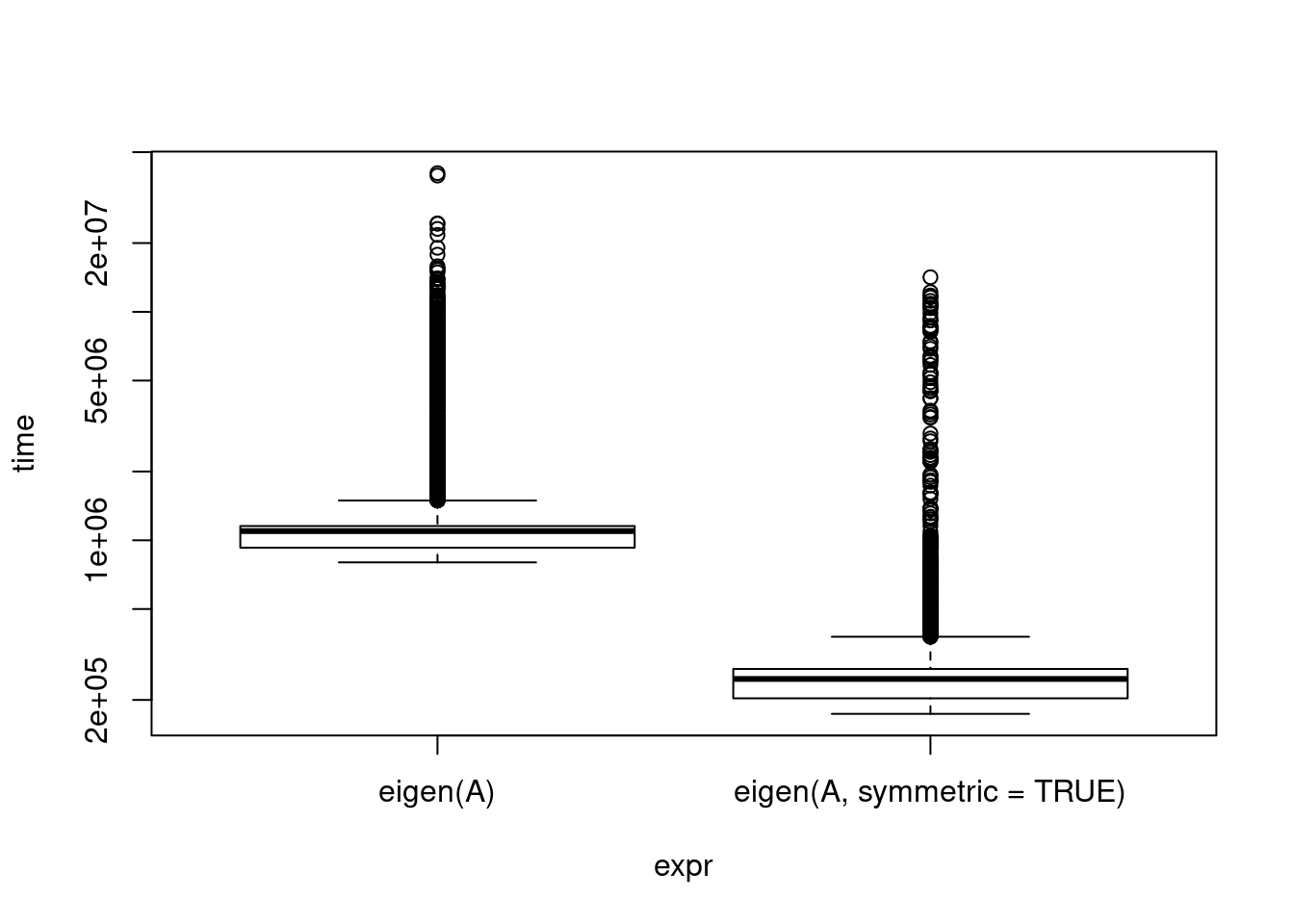
I noticed this when I was profiling my code for something that did, unfortunately, require both eigenvalues and matrix inversion. profvis indicated eigen() was a big drag on my speed, but when I drilled down, I saw much of it was spent on isSymmetric() (verify yourself, R Studio makes it easy!). My input was a covariance matrix so it was guaranteed to be symmetric. Reading the helpful manual page, I saw that the argument can be provided. Unfortunately, reading the source code, they drop down into C to compute the eigenvalues, so there isn’t an additional chance for speedup there.
Let’s return to the first example: we are dealing with a covariance matrix, so there are other ideas besides (the disastrous) qr.solve available.
cholinv <- microbenchmark(
  solve(A, B), # worked best last time
  solve(A) %*% B,
  chol2inv(chol(A)) %*% B,
  times = 1e4
)
print(cholinv)
Unit: microseconds
expr min lq mean median uq
solve(A, B) 54.450 58.8080 73.00514 67.5460 78.9180
solve(A) %*% B 78.507 83.5035 109.63726 101.5195 117.4545
chol2inv(chol(A)) %*% B 39.675 46.0860 60.70087 51.5485 68.9265
max neval
6957.469 10000
4529.604 10000
4262.751 10000Reuse information
Nothing above really stood out, except what we learned before. Calculating the Cholesky decomposition is on the same order of complexity as solving and ends up having about the same runtime - it’s slightly better, but nothing to write home about. However, suppose for some reason you already have the Cholesky decomposition (note: always check notation - some people use the term for \(L\) such that \(LL^T = X\) and some use it for \(R\) such that \(R^T R = X\) - which does R use?).
C <- chol(A)
cholinv <- microbenchmark(
  solve(A, B), # worked best last time
  chol2inv(C) %*% B,
  times = 1e4
)
print(cholinv)
Unit: microseconds
expr min lq mean median uq max neval
solve(A, B) 55.271 59.090 80.50626 68.7105 77.9850 90785.951 10000
chol2inv(C) %*% B 16.399 18.088 23.53046 20.5790 27.5755 3426.222 10000plot(cholinv, log = "y")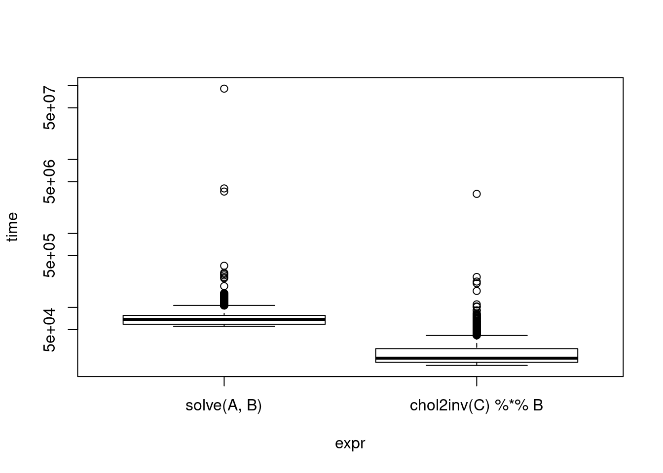
There is a similar idea if you already happen to have the results of eigen() on hand. Cutting time in half is a decent result.
Determinants
One good reason to have a Cholesky decomposition or eigenvalue decomposition on hand (besides the fun of it) is to avoid computing a determinant, which comes up in densities all the time. Again, since we’re looking at a covariance matrix, there are ways around direct computation. Both of these are unfortunately of the same order of complexity as computing a determinant but slightly faster. However, if you need a determinant, you just might also need the eigenvalues or the Cholesky decomposition or an inverse. If that is the case, what were once modest gains in speed become big savings.
detbenchmark <- microbenchmark(
  det(A),
  prod(diag((chol(A))))^2,
  prod(diag(C))^2, # C = chol(A)
  prod(eigen(A, symmetric = TRUE)$values),
  prod(eigenA$values) # eigenA = eigen(A)
)
print(detbenchmark)
Unit: microseconds
expr min lq mean
det(A) 32.682 38.3810 53.52603
prod(diag((chol(A))))^2 36.341 47.0790 57.75653
prod(diag(C))^2 9.312 11.3220 15.09580
prod(eigen(A, symmetric = TRUE)$values) 183.987 194.2880 233.88735
prod(eigenA$values) 4.531 6.2545 7.69604
median uq max neval
45.2120 58.1330 413.135 100
50.9905 69.7050 112.526 100
13.3870 16.8630 45.312 100
220.5430 267.7650 327.987 100
7.1770 8.7485 30.237 100Again, we see that while performing a decomposition just for the sake of computing something faster may not be worth it, it’s worth keeping in mind that if you need multiple things, doing so may be much faster, and if you need one of these anyway, keep the result and use it for the others. These will also vary based on your use cases, so profiling is the best idea.
What brought this up
A project where I needed Cholesky decompositions, inverses, and sometimes even determinants or eigenvalues as well. I’m not trying to be fast, but it’s nice to not be terribly slow. Again, if you don’t need more than one of the above, don’t bother! Wasting developer time is rarely worth it. If you have more specialized needs, of course, there are other tools for that.
NB: of course you want to validate that you get the same answers and if applicable add them as test cases in your computations.