Why don't my results agree with some other function?

Or even with other functions in the same package? With a set seed, one would expect the random draws from two equivalent distributions to be the same.

library('MixMatrix')
set.seed(20180223)
rmatrixnorm(n = 1, mean = matrix(0, nrow = 1, ncol = 5), array = T)

## , , 1
## 
##          [,1]        [,2]     [,3]      [,4]         [,5]
## [1,] 1.153053 -0.08006347 1.040504 0.9671611 -0.002402098

set.seed(20180223)
rmatrixnorm(n = 1, mean = matrix(0, nrow = 5, ncol = 1), array = T)

## , , 1
## 
##              [,1]
## [1,]  1.153052900
## [2,] -0.080063466
## [3,]  1.040504256
## [4,]  0.967161119
## [5,] -0.002402098

set.seed(20180223)
rnorm(5)

## [1]  1.153052900 -0.080063466  1.040504256  0.967161119 -0.002402098

However, this breaks when we try it with the \(t\)-distribution.

set.seed(20180223)
rmatrixt(n = 1, df = 5, mean = matrix(0, nrow = 1, ncol = 5))

##           [,1]        [,2]      [,3]      [,4]         [,5]
## [1,] 0.5556109 -0.03857944 0.5013781 0.4660369 -0.001157477

set.seed(20180223)
rmatrixt(n = 1, df = 5, mean = matrix(0, nrow = 5, ncol = 1))

##            [,1]
## [1,] 0.80490445
## [2,] 0.04992909
## [3,] 0.38812672
## [4,] 0.96679126
## [5,] 0.33254232

What is going on here?

It is not because the densities are calculated differently or the distributions are different.

x = matrix(1, nrow=5, ncol=1)
dmatrixt(x, df = 5)

## [1] 0.0001327224

dmatrixt(t(x), df = 5)

## [1] 0.0001327224

A <- t(drop(rmatrixt(n = 1e5, df = 5, mean = matrix(0, nrow = 1, ncol = 5))))
B <- t(drop(rmatrixt(n = 1e5, df = 5, mean = matrix(0, nrow = 5, ncol = 1))))
var(A)

##               [,1]          [,2]         [,3]          [,4]         [,5]
## [1,]  0.3376941545 -0.0026526140 -0.003364226  0.0002350722  0.001506509
## [2,] -0.0026526140  0.3392196610  0.002651327 -0.0001851677 -0.004766983
## [3,] -0.0033642256  0.0026513274  0.332201222 -0.0012015348  0.001478222
## [4,]  0.0002350722 -0.0001851677 -0.001201535  0.3336451673 -0.002856316
## [5,]  0.0015065085 -0.0047669830  0.001478222 -0.0028563164  0.332690166

var(B)

##               [,1]          [,2]          [,3]          [,4]          [,5]
## [1,]  0.3308014396 -0.0014946855  0.0028350338 -0.0008405594  0.0006931611
## [2,] -0.0014946855  0.3289382913  0.0017313093  0.0004647432  0.0031412509
## [3,]  0.0028350338  0.0017313093  0.3324019321 -0.0001002768  0.0026761169
## [4,] -0.0008405594  0.0004647432 -0.0001002768  0.3343747962 -0.0037769019
## [5,]  0.0006931611  0.0031412509  0.0026761169 -0.0037769019  0.3338379308

In fact, if we look at rmvt from the excellent mvtnorm package, we can see that one of them agrees with their function.

library('mvtnorm')
set.seed(20180223)
rmatrixt(n = 1, df = 5, mean = matrix(0, nrow = 1, ncol = 5))

##           [,1]        [,2]      [,3]      [,4]         [,5]
## [1,] 0.5556109 -0.03857944 0.5013781 0.4660369 -0.001157477

set.seed(20180223)
rmvt(1,sigma=.2*diag(5), df = 5) # note that matrix t is scaled by DF compared to multivariate t

##           [,1]        [,2]      [,3]      [,4]         [,5]
## [1,] 0.5556109 -0.03857944 0.5013781 0.4660369 -0.001157477

What is going on

Here is a hint as to what is happening from the source code of rmvt:

rmvnorm(n, mean = delta, sigma = sigma, ...)/sqrt(rchisq(n, 
            df)/df)

It draws from the multivariate normal distribution and then scales by individual draws from rchisq. This is essentially what happens in rmatrixt as well when the dimension of \(U\) (the number of rows) is \(1\). The matrix version takes the Cholesky factor of an inverse Wishart draw, which in the 1-dimensional case is the inverse of the square root of a draw from rchisq.

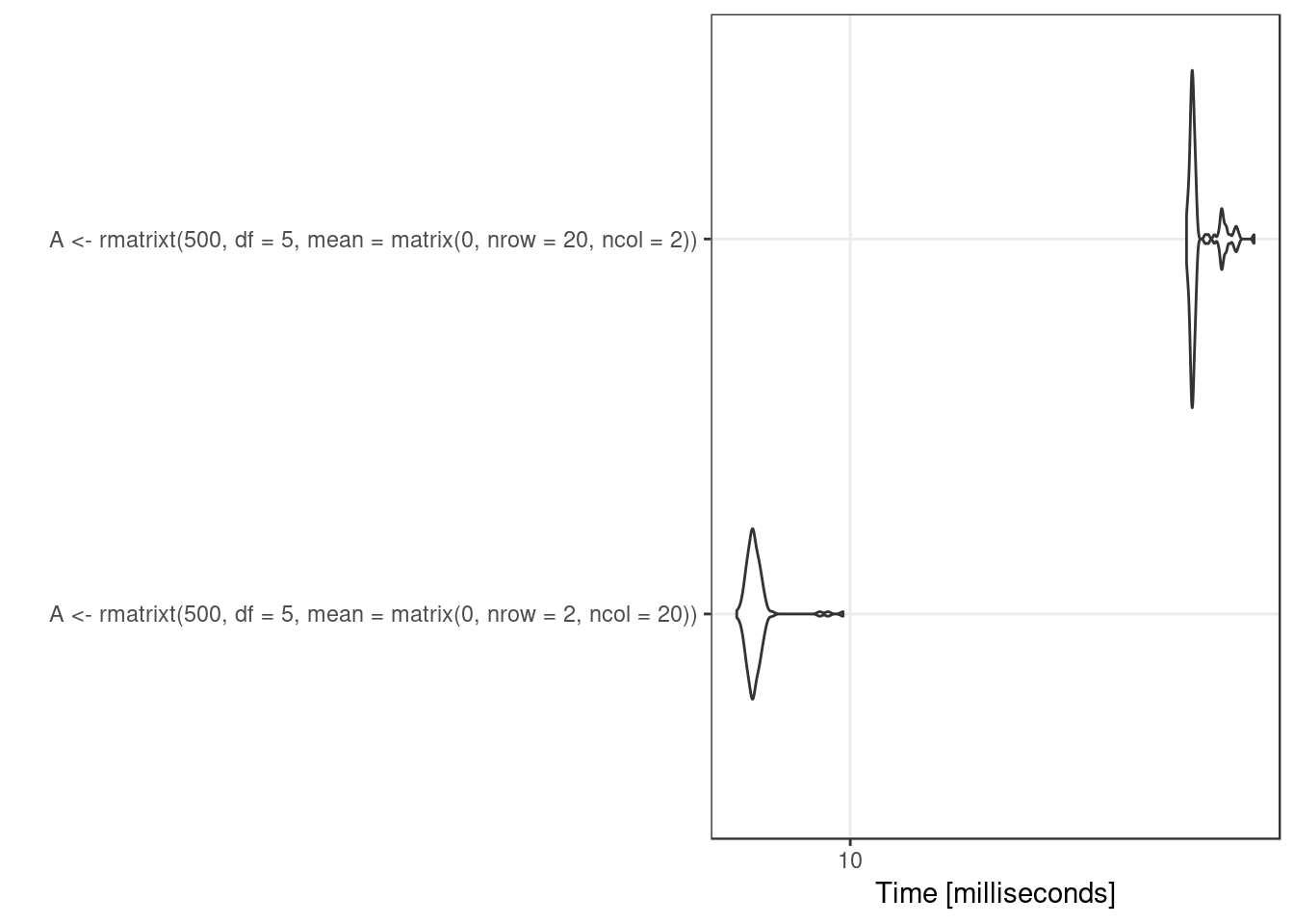
However, when the dimension (\(p\)) of \(U\) is larger than \(1\), the multiplicative factor is not the same, it is the Cholesky factor of an inverse Wishart draw of dimension \(p\), which involves drawing \(p\) rchisq and choose(p, 2)-p draws from rnorm. The densities end up the same but the computation involves such different numbers there is no hope of getting the same numbers. Further, this suggests that, when drawing from matrix variate \(t\)-distributions, given that \(X\) and \(X'\) have the same distributions, care should be taken so that the faster direction for simulation is used.

library('microbenchmark')
res <- microbenchmark(
A <- rmatrixt(500, df = 5, mean = matrix(0, nrow = 2, ncol = 20)),
A <- rmatrixt(500, df = 5, mean = matrix(0, nrow = 20, ncol = 2))
)
print(res)

## Unit: milliseconds
##                                                               expr       min
##  A <- rmatrixt(500, df = 5, mean = matrix(0, nrow = 2, ncol = 20))  7.064598
##  A <- rmatrixt(500, df = 5, mean = matrix(0, nrow = 20, ncol = 2)) 20.527809
##         lq      mean    median        uq      max neval
##   7.208044  8.205559  7.382543  8.432845 13.62678   100
##  20.743099 21.985216 21.060493 22.251205 35.50845   100

library('ggplot2')
autoplot(res) + theme_bw()

## Coordinate system already present. Adding new coordinate system, which will replace the existing one.